GETTING STARTED
- Open the file1.xlsx, available for download from the SAM website.
- Save the file as.xlsx by changing the “1” to a “2”.
- If you do not see the 2.xlsx file extension in the Save As dialog box, do not type it. The program will add the file extension for you automatically.
- With the file 2.xlsx still open, ensure that your first and last name is displayed in cell B6 of the Documentation sheet.
- If cell B6 does not display your name, delete the file and download a new copy from the SAM website.
PROJECT STEPS
- Stella Scott has a work-study position at the fitness center on campus. Her manager has asked her to create a worksheet to keep track of attendance and revenue for the fitness center’s classes.
Open the Class Statistics worksheet. Modify the column widths and row heights as described below:
- Use AutoFit to change the width of column A to make all the contents visible.
- Change the row height of row 1 to 42.00 pts.
- Change the widths of columns B through M to 10.25 characters.
- In the merged range A1:M1, apply the formatting options described below:
- Change the font to Tw Cen MT and the font size to 26 pt.
- Change the font color to Turquoise, Accent 3, Darker 50% (7th column, 6th row of the Theme Colors palette).
- Change the fill color of the cell to Turquoise, Accent 3, Lighter 80% (7th column, 2nd row of the Theme Colors palette).
- Use Merge Cells to mergethe contents of the range A2:M2 and then apply the Heading 1 cell style to the merged range. Format the merged range with the Short Date number format.
- Enter the contents in bold shown in Table 1 below into the range C4:G5.
Table 1: Data for Range C4:G5
| C | D | E | F | G | |
| 4 | Cardio | Hip-Hop | Spinning | Yoga | Zumba |
| 5 | 100 | 150 | 120 | 200 | 150 |
- Format the cells in the range C5:G5 with the Currency number format with two decimal places and $ as the symbol.
- Apply the following formatting options, as described below:
- Bold and center the content of cell B4.
- Use the Format Painter to copy the formatting of cell B4 to the range C4:G4.
- Use Merge Cells to merge the contents of the range B4:B5.
- Apply the All Borders border style to the range B4:G5.
- Move the content of cell H6 to cell G7 and then apply the formatting options described below:
- Merge and center the range G7:K7.
- Apply the fill color Blue, Accent 2, Lighter 60% (6th column, 3rd row of the Theme Colors palette) to the merged range.
- Use the September label in cell B8 to fill the range C8:M8 with the months of the year.
- In cell B14, use the SUM function to total the values in the range B9:B13. Use the Fill handle to copy the formula from B14 into the range C14:M14.
- In January, the hip-hop class is the center’s least attended class, but Stella’s manager hopes to boost attendance so that they can reach their budget goals.
Perform a Goal Seek analysis to determine the number of hip-hop class attendees needed in January (F10) to change the value in cell F14 to 400. (Hint: Cell F10 will be the changing cell.) Keep the results of the Goal Seek Analysis as the new value for cell F10.
- In cell B15, use the keyboard to enter a formula that multiplies the value in cell B9 (the number of students attending the cardio class) by the value in cell C5 (the cost of each cardio class). Use an absolute cell reference to cell C5 and a relative reference to cell B9. Copy the formula from cell B15 to the range C15:M15.
- Calculate the revenue for the two remaining unfilled classes (Yoga and Zumba) as described below, using absolute references to the cells in the range F5:G5:
- In cell B18, enter a formula that multiples the value in cell B12 by the value in cell F5. Copy the formula from B18 to the range C18:M18.
- In cell B19, enter a formula that multiples the value in cell B13 by the value in cell G5. Copy that formula from B19 to the range C19:M19.
- Format the values in the range B9:M14 with the Comma Style number format with zero decimal places. Format the range B15:M20 with the Accounting number format with two decimal places.
- To help see where the most profitable months are, apply a new conditional formatting rule to the range B20:M20. The rule should format only cells that contain cell values greater than $62,000 with Light Green fill color (5th column, 1st row of the Standard Colors palette) and Dark Blue font color (9th column, 1st row of the Standard Colors palette).
- In cell B23, use the AVERAGE function to calculate the average monthly revenue generated for the range B15:B19. Copy the formula from cell B23 to the range C23:M23.
- In cell B24, use the MAX function to calculate which value in the range B15:B19 is the largest. Copy the formula from cell B24 to the range C24:M24.
- In cell B25, use the MIN function to calculate which value in the range B15:B19 is the smallest. Copy the formula from cell B25 to the range C25:M25.
- The center needs to bring in $13,400 a month to stay on budget. In cell B26, use the IF function to check whether the value of cell B23 is greater than 13,400.
- If this condition is true, the cell value should be set to Over (Hint: For the value if true, use “Over”).
- If this condition is false, the cell value should be set to Under (Hint: For the value if false, use “Under”).
Copy the formula created in cell B26 to the range C26:M26.
- In cell B28, create a Line Sparkline from the data in the range G11:K11, and then change the style of the Sparkline to Turquoise, Sparkline Style Accent 3 (no dark or light). (Hint: Depending on your version of Office, the sparkline style may be written as Sparkline Style Accent 3 (no dark or light).)
- Check the Spelling in the workbook to identify and correct any spelling errors. (Hint: You should find and correct at least two spelling errors.)
- Format the worksheet for printing as described below:
- Change the orientation to Landscape.
- Change the worksheet margins to Narrow.
- Insert a header in the center section with the text 2018 Class Statistics.
- Scale the worksheet so that it prints on one page.
Switch back to Normal View.
- Stella’s manager would like to emphasize certain visuals in the worksheet.
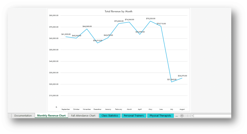
Create a Line chart from the nonadjacent ranges B8:M8 and B20:M20. Move the chart you just created to its own chart sheet. Use Monthly Revenue Chart as the name of the new chart sheet.
- On the Monthly Revenue Chart worksheet, format the line chart with the following options:
- Change the chart title to Total Revenue by Month.
- Format the data labels using the Above positioning option.
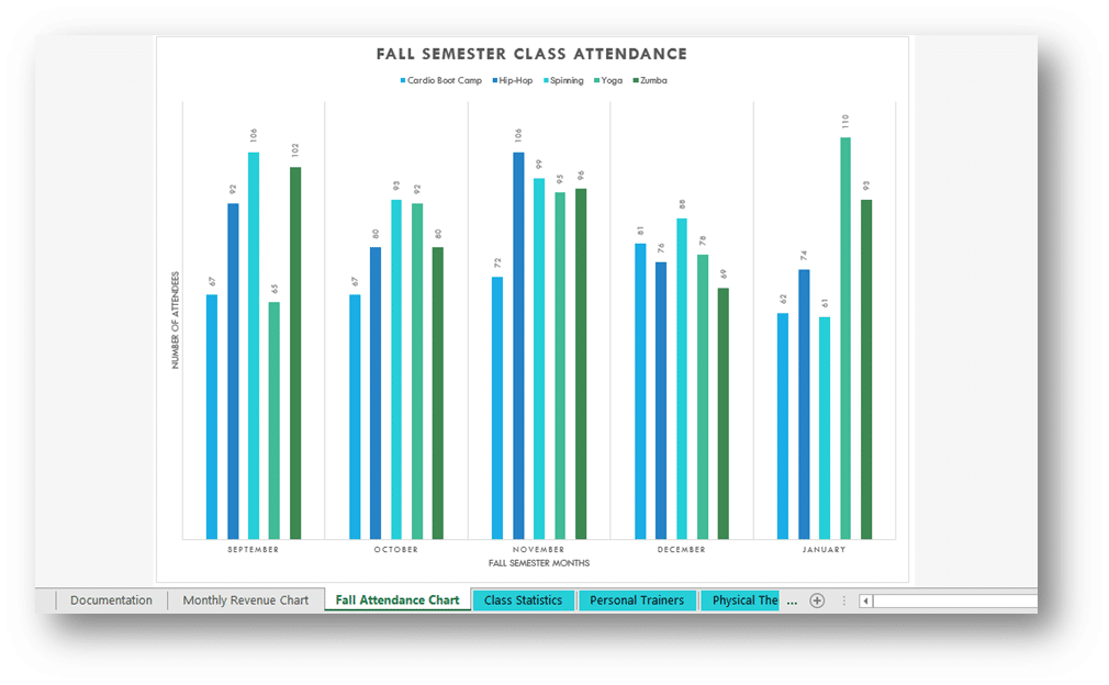
- Switch back to the Class Statistics worksheet. Use the Recommended Chart tool to create a Clustered Column chart based on the range A8:F13. Move the chart to its own chart sheet. Use the name Fall Attendance Chart as the name of the new chart sheet.
- On the Fall Attendance Chart chart sheet, format the clustered column chart with the following options:
- Change the chart style to Chart Style 2.
- Change the chart title to Fall Semester Class Attendance.
- Add Number of Attendees as the primary vertical axis title.
- Add Fall Semester Months as the primary horizontal axis title.
- Stella’s manager was very impressed with her work and would like her to include and format some other information as well.
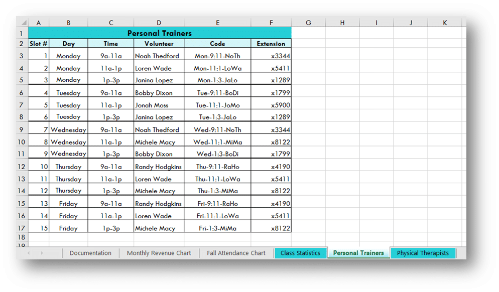
Go to the Personal Trainers worksheet and make the following formatting changes:
- Rotate the labels in the range B3:B17 to 0 degrees.
- Copy the range C3:C5, then paste it into the range C6:C17. Use the paste option that pastes the values, but not the cell formatting.
- Set the fill color in cell C3 and the range D6:D8 to No Fill.
- The center uses special codes to keep track of hours and process payments. These codes are made by typing the first three letters of the day followed by a dash, the start and end times separated by a colon, a dash, and then the first two letters of the first and last name of the trainer.
In cell E4, type Mon-11:1-LoWa. Select the range E3:E17, and use Flash Fill to fill the values in the range.
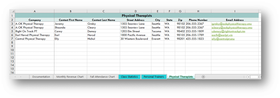
- In the Physical Therapists worksheet, select cell B3 and use the Freeze Panes option to freeze the rows and columns above and to the left of cell B3.
- Select the Class Statistics, Personal Trainers, and Physical Therapists worksheets and then change the color of the sheet tabs to Turquoise, Accent 3 (7th column, 1st row of the Theme Colors palette).
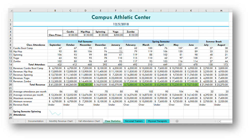
Your workbook should look like the Final Figures on the following pages. (The value in cell F10 generated by the Goal Seek analysis has intentionally been blurred out in Final Figure 3.) Save your changes, close the workbook, and then exit Excel. Follow the directions on the SAM website to submit your completed project.
Final Figure 1: Monthly Revenue Chart Worksheet
Final Figure 2: Fall Attendance Chart Worksheet
Final Figure 3: Class Statistics Worksheet
Final Figure 4: Personal Trainers Worksheet
Final Figure 5: Physical Therapists Worksheet
Do you need urgent help with this or a similar assignment? We got you. Simply place your order and leave the rest to our experts.
